Chapter 8 Complexity regularization
8.1 Bias-variance tradeoff
To set the stage for the remainder of this note we will briefly revisit the bias-variance trade-off in this section. In particular we will illustrate the effect of varying the sample size \(n\). Readers familiar with this topic may choose to skip this section.
As as in Bishop (2006) we consider synthetic data generated by the sinusoidal function \(f(x)=\sin(2\pi x)\). To simulate random samples of \(\mathbf{y}\) we sample \(n\) input values from \(\mathbf{X} \sim \text{unif}(0,1)\) and introduce a random noise component \(\varepsilon \sim \mathcal{N}(0,0.3)\). Figure 8.1 shows \(\mathbf{y}\) along with random draws \(\mathbf{y}^*_n\).
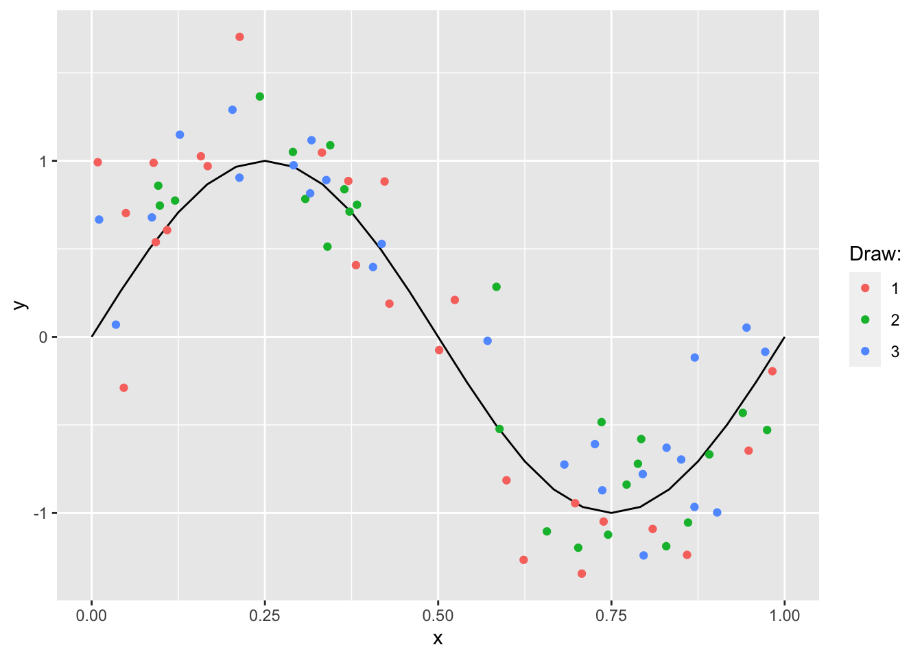
Figure 8.1: Sinusoidal function and random draws.
Following Bishop (2006) we will use a Gaussian linear model with Gaussian kernels \(\exp(-\frac{(x_k-\mu_p)^{2}}{2s^2})\) as
\[ \begin{equation} \begin{aligned} && \mathbf{y}|\mathbf{X}& =f(x) \sim \mathcal{N} \left( \sum_{j=0}^{p-1} \phi_j(x)\beta_j, v \mathbb{I}_p \right) \\ \end{aligned} \tag{8.1} \end{equation} \]
with \(v=0.3\) to estimate \(\hat{\mathbf{y}}_k\) from random draws \(\mathbf{X}_k\). We fix the number of kernels \(p=24\) (and hence the number of features \(M=p+1=25\)) as well as the spatial scale \(s=0.1\). To vary the complexity of the model we use a form of regularized least-squares (Ridge regression) and let the regularization parameter \(\lambda\) vary
\[ \begin{equation} \begin{aligned} && \hat\beta&=(\lambda I + \Phi^T \Phi)^{-1}\Phi^Ty \\ \end{aligned} \tag{8.2} \end{equation} \]
where high values of \(\lambda\) in (8.2) shrink parameter values towards zero. (Note that a choice \(\lambda=0\) corresponds to the OLS estimator which is defined as long as \(p \le n\).)
As in Bishop (2006) we proceed as follows for each choice of \(\lambda\) and each sample draw to illustrate the bias-variance trade-off:
- Draw \(N=25\) time from \(\mathbf{u}_k \sim \text{unif}(0,1)\).
- Let \(\mathbf{X}_k^*=\mathbf{u}_k+\varepsilon_k\) with \(\varepsilon \sim \mathcal{N}(0, 0.3)\).
- Compute \(\mathbf{y}_k^*=\sin(2\pi \mathbf{X}^*_k)\).
- Extract features \(\Phi_k\) from \(\mathbf{X}_k^*\) and estimate the parameter vector \(\beta_k^*(\Phi_k,\mathbf{y}^*_k,\lambda)\) through regularized least-squares.
- Predict \(\hat{\mathbf{y}}_k^*=\Phi \beta_k^*\).
Applying the above procedure we can construct the familiar picture that demonstrates how increased model complexity increases variance while reducing bias (Figure 8.2). Recall that for the mean-squared error (MSE) we have
\[ \begin{equation} \begin{aligned} && \mathbb{E} \left( (\hat{f}_n(x)-f(x))^2 \right) &= \text{var} (\hat{f}_n(x)) + \left( \mathbb{E} \left( \hat{f}_n(x) \right) - f(x) \right)^2 \\ \end{aligned} \tag{2.1} \end{equation} \]
where the first term on the right-hand side corresponds to the variance of our prediction and the second term to its (squared) bias. In Figure 8.2 as model complexity increases the variance component of the MSE increases, while the bias term diminishes. A similar pattern would have been observed if instead of using regularization we had used OLS and let the number of Gaussian kernels (and hence the number of features \(p\)) vary where higher values of \(p\) correspond to increased model complexity.
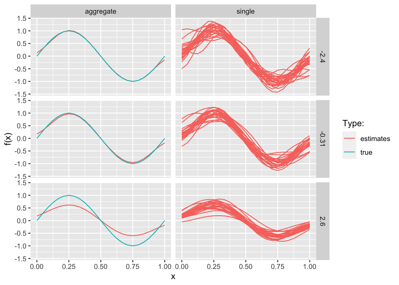
Figure 8.2: Bias-variance trade-off