Chapter 10 Subsampling
When working with very large sample data, even the estimation of ordinary least-squares can be computationally prohibitive. Since we increasingly find ourselves in situations where the sample size \(n\) is extremely high, a body of literature concerned with optimal subsampling has recently emerged. This post summarises some of the main ideas and methodologies that have emerged from that literature. This chapter is structured as follows: the first section briefly revisits the bias-variance trade-off already introduced in Chapter 8.1. The following section then introduces various subsampling methods. Section 10.3 illustrates the improvements associated with non-uniform subsampling. The final two sections apply the developed ideas to binary classification problems with imbalanced training data. Section 10.5 concludes.
10.1 Motivation
Recall the discussion of bias-variance trade-off in Chapter 8.1 where we showed that as model complexity increases the variance component of the mean-squared error increases, while the bias term diminishes. The focus here is instead on varying the sample size \(n\). It should not be surprising that both the variance and bias component of the MSE decrease as the sample size \(n\) increases (Figure 10.1). But in today’s world \(n\) can potentially be very large, so much so that even computing simple linear models can be hard. Suppose for example you wanted to use patient data that is generated in real-time as a global pandemic unfolds to predict the trajectory of said pandemic. Or consider the vast quantities of potentially useful user-generated data that online service providers have access to. In the remainder of this note we will investigate how systematic subsampling can help improve model accuracy in these situations.
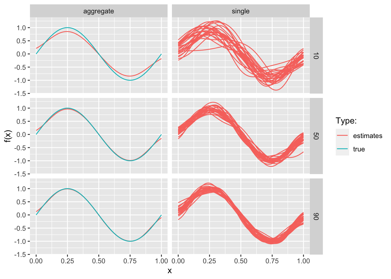
Figure 10.1: Bias-variance trade-off
10.2 Subsampling methods
The case for subsampling generally involves \(n >> p\), so very large values of \(n\). In such cases we may be interested in estimating \(\hat\beta_m\) instead of \(\hat\beta_n\) where \(p\le m<<n\) with \(m\) freely chosen by us. In practice we may want to do this to avoid high computational costs associated with large \(n\) as discussed above. The basic algorithm for estimating \(\hat\beta_m\) is simple:
- Subsample with replacement from the data with some sampling probability \(\{\pi_i\}^n_{i=1}\).
- Estimate least-squares estimator \(\hat\beta_m\) using the subsample.
But there are at least two questions about this algorithm: firstly, how do we choose \(\mathbf{X}_m=({\mathbf{X}^{(1)}}^T,...,{\mathbf{X}^{(m)}}^T)^T\)? Secondly, how should we construct \(\hat\beta_m\)? With respect to the former, a better idea than just randomly selecting \(\mathbf{X}_m\) might be to choose observations with high influence. We will look at a few of the different subsampling methods investigated and proposed in Zhu et al. (2015), which differ primarily in their choice of subsampling probabilities \(\{\pi_i\}^n_{i=1}\):
- Uniform subsampling (UNIF): \(\{\pi_i\}^n_{i=1}=1/n\).
- Basic leveraging (BLEV): \(\{\pi_i\}^n_{i=1}=h_{ii}/ \text{tr}(\mathbf{H})=h_{ii}/p\) where \(\mathbf{H}\) is the hat matrix.
- Optimal (OPT) and predictor-length sampling (PL): involving \(||\mathbf{X}_i||/ \sum_{j=1}^{n}||\mathbf{X}_j||\) where \(||\mathbf{X}||\) denotes the \(L_2\) norm of \(\mathbf{X}\).
Methods involving predictor-lengths are proposed by the authors with the former shown to be optimal (more on this below). PL subsampling is shown to scale very well and a good approximation of optimal subsampling conditional on leverage scores \(h_{ii}\) being fairly homogeneous.
With respect to the second question Zhu et al. (2015) investigate both ordinary least-squares (OLS) and weighted least-squares (WLS). With respect to the latter the weights we need to supply to the ols function introduced in Chapter 7.1 are simply \(w=\{1/\pi_i\}^m_{i=1}\). This follows from the following property of diagonal matrices:
\[ \begin{aligned} && \Phi^{-1}&= \begin{pmatrix} 1\over\phi_{11} & 0 & 0 \\ 0 & ... & 0 \\ 0 & 0 & 1\over \phi_{nn} \end{pmatrix} \\ \end{aligned} \]
The authors present empirical evidence that OLS is more efficient than WLS in that the mean-squared error (MSE) for predicting \(\mathbf{X} \beta\) is lower for OLS. The authors also note though that subsampling using OLS is not consistent for non-uniform subsampling methods meaning that the bias cannot be controlled. Given Equation (2.1) the fact that OLS is nonetheless more efficient than WLS implies that the higher variance terms associated with WLS dominates the effect of relatively higher bias with OLS. In fact this is consistent with the theoretical results presented in Zhu et al. (2015) (more on this below).
Next we will briefly run through different estimation and subsampling methods in some more detail and see how they can be implemented in R. In the following section we will then look at how the different approaches perform empirically.
10.2.1 Uniform subsampling (UNIF)
A simple function for uniform subsampling in R is shown in the code chunk below. Note that to streamline the comparison of the different methods in the following section the function takes an unused argument weighted=F which for the other subsampling methods can be used to determine whether OLS or WLS should be used. Of course, with uniform subsampling the weights are all identical and hence \(\hat\beta^{OLS}=\hat\beta^{WLS}\) so the argument is passed to but not evaluated in sub_UNIF.
function (X, y, m, weighted = F, rand_state = NULL)
{
    if (!is.null(rand_state)) {
        set.seed(rand_state)
    }
    indices <- sample(1:n, size = m)
    X_m <- X[indices, ]
    y_m <- y[indices]
    beta_hat <- qr.solve(X_m, y_m)
    y_hat <- c(X %*% beta_hat)
    return(list(fitted = y_hat, coeff = beta_hat))
}
10.2.2 Basic leveraging (BLEV)
The sub_UNIF function can be extended easily to the case with basic leveraging (see code below). Note that in this case the weighted argument is evaluated.
function (X, y, m, weighted = F, rand_state = NULL, plot_wgts = F, prob_only = F)
{
    svd_X <- svd(X)
    U <- svd_X$u
    H <- tcrossprod(U)
    h <- diag(H)
    prob <- h/ncol(X)
    if (plot_wgts) {
        plot(prob, t = "l", ylab = "Sampling probability")
    }
    if (prob_only) {
        return(prob)
    }
    else {
        indices <- sample(x = 1:n, size = m, replace = T, prob = prob)
        X_m <- X[indices, ]
        y_m <- y[indices]
        weights <- 1/prob[indices]
        if (weighted) {
            beta_hat <- wls_qr(X_m, y_m, weights)
        }
        else {
            beta_hat <- qr.solve(X_m, y_m)
        }
        y_hat <- c(X %*% beta_hat)
        return(list(fitted = y_hat, coeff = beta_hat, prob = prob))
    }
}
10.2.2.1 A note on computing leverage scores
Recall that for the hat matrix we have
\[ \begin{equation} \begin{aligned} && \mathbf{H}&=\mathbf{X} (\mathbf{X}^T \mathbf{X})^{-1}\mathbf{X}^T \\ \end{aligned} \tag{10.1} \end{equation} \]
where the diagonal elements \(h_{ii}\) correspond to the leverage scores we’re after. Following Zhu et al. (2015) we will use (compact) singular value decomposition to obtain \(\mathbf{H}\) rather than computing (10.1) directly. This has the benefit that there exist exceptionally stable numerical algorithms to compute SVD. To see how and why we can use SVD to obtain \(\mathbf{H}\) see appendix.
Clearly to get \(h_{ii}\) we first need to compute \(\mathbf{H}\) which in terms of computational costs is of order \(\mathcal{O}(np^2)=\max(\mathcal{O}(np^2),\mathcal{O}(p^3))\). The fact that we use all \(n\) rows of \(\Phi\) to compute leverage scores even though we explicitly stated our goal was to only use \(m\) observations may rightly seem like a bit of a paradox. This is why fast algorithms that approximate leverage scores have been proposed. We will not look at them specifically here mainly because the PL method proposed by Zhu et al. (2015) does not depend on leverage scores and promises to be computationally even more efficient.
10.2.3 Predictor-length sampling (PL)
The basic characteristic of PL subsampling - choosing \(\{\pi_i\}^n_{i=1}= ||\mathbf{X}_i||/ \sum_{j=1}^{n}||\mathbf{X}_j||\) - was already introduced above. Again it is very easy to modify the subsampling functions from above to this case:
function (X, y, m, weighted = F, rand_state = NULL, plot_wgts = F, prob_only = F)
{
    predictor_len <- sqrt(X^2 %*% rep(1, ncol(X)))
    prob <- predictor_len/sum(predictor_len)
    if (plot_wgts) {
        plot(prob, t = "l", ylab = "Sampling probability")
    }
    if (prob_only) {
        return(prob)
    }
    else {
        indices <- sample(x = 1:n, size = m, replace = T, prob = prob)
        X_m <- X[indices, ]
        y_m <- y[indices]
        weights <- 1/prob[indices]
        if (weighted) {
            beta_hat <- wls_qr(X_m, y_m, weights)
        }
        else {
            beta_hat <- qr.solve(X_m, y_m)
        }
        y_hat <- c(X %*% beta_hat)
        return(list(fitted = y_hat, coeff = beta_hat, prob = prob))
    }
}
10.2.3.1 A note on optimal subsampling (OPT)
In fact, PL subsampling is an approximate version of optimal subsampling (OPT). Zhu et al. (2015) show that asymptotically we have:
\[ \begin{equation} \begin{aligned} &&\text{plim} \left( \text{var} (\hat{f}_n(x)) \right) > \text{plim} \left(\left( \mathbb{E} \left( \hat{f}_n(x) \right) - f(x) \right)^2 \right) \\ \end{aligned} \tag{10.2} \end{equation} \]
Given this result minimizing the MSE (Equation (2.1)) with respect to subsampling probabilities \(\{\pi_i\}^n_{i=1}\) corresponds to minimizing \(\text{var} (\hat{f}_n(x))\). They further show that this minimization problem has the following closed-form solution:
\[ \begin{equation} \begin{aligned} && \pi_i&= \frac{\sqrt{(1-h_{ii})}||\mathbf{X}_i||}{\sum_{j=1}^n\sqrt{(1-h_{jj})}||\mathbf{X}_j||}\\ \end{aligned} \tag{10.3} \end{equation} \]
This still has computational costs of order \(\mathcal{O}(np^2)\). But it should now be clear why PL subsampling is optimal conditional on leverage scores being homogeneous (see appendix). PL subsampling is associated with computational costs of order \(\mathcal{O}(np)\), so a potentially massive improvement. The code for optimal subsampling is shown below:
function (X, y, m, weighted = F, rand_state = NULL, plot_wgts = F, prob_only = F)
{
    n <- nrow(X)
    svd_X <- svd(X)
    U <- svd_X$u
    H <- tcrossprod(U)
    h <- diag(H)
    predictor_len <- sqrt(X^2 %*% rep(1, ncol(X)))
    prob <- (sqrt(1 - h) * predictor_len)/crossprod(sqrt(1 - h), predictor_len)[1]
    if (plot_wgts) {
        plot(prob, t = "l", ylab = "Sampling probability")
    }
    if (prob_only) {
        return(prob)
    }
    else {
        indices <- sample(x = 1:n, size = m, replace = T, prob = prob)
        X_m <- X[indices, ]
        y_m <- y[indices]
        weights <- 1/prob[indices]
        if (weighted) {
            beta_hat <- wls_qr(X_m, y_m, weights)
        }
        else {
            beta_hat <- qr.solve(X_m, y_m)
        }
        y_hat <- c(X %*% beta_hat)
        return(list(fitted = y_hat, coeff = beta_hat, prob = prob))
    }
}
10.2.3.2 A note on computing predictor lengths
Computing the Euclidean norms \(||\mathbf{X}_i||\) in R can be done explicitly by looping over the rows of \(\mathbf{X}\) and computing the norm in each iteration. It turns out that this computationally very expensive. A much more efficient way of computing the vector of predictor lengths is as follows
\[ \begin{equation} \begin{aligned} && \mathbf{pl}&=\sqrt{\mathbf{X}^2 \mathbf{1}} \\ \end{aligned} \tag{10.4} \end{equation} \]
where \(\mathbf{X}^2\) indicates elements squared, the square root is also taken element-wise and \(\mathbf{1}\) is a \((p \times 1)\) vectors of ones. A performance benchmark of the two approaches is shown in Figure 10.2 below.
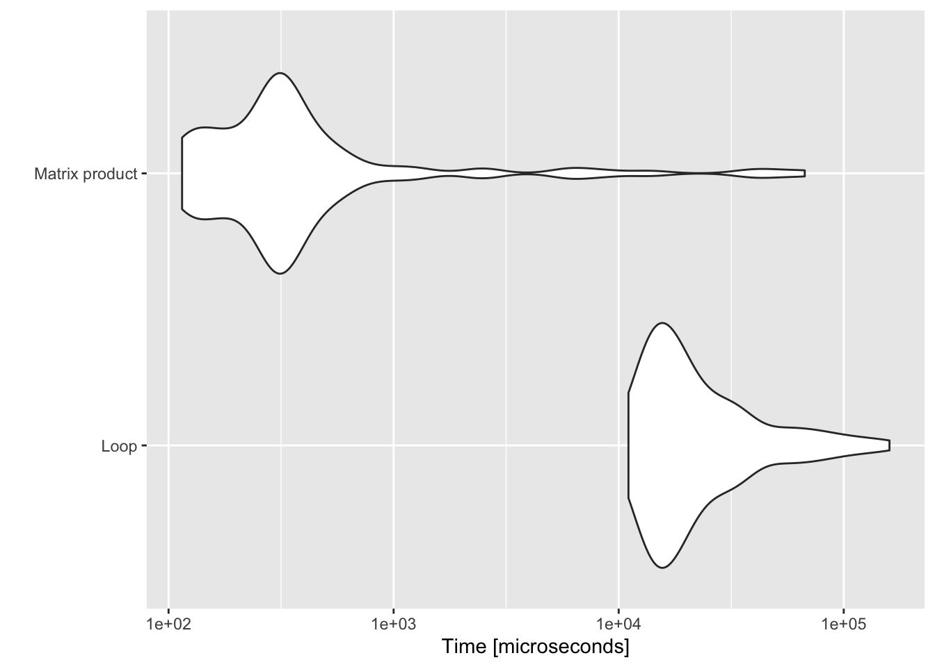
Figure 10.2: Benchmark of Euclidean norm computations.
10.2.4 Comparison of methods
As discussed in Zhu et al. (2015) both OPT and PL subsampling tend to inflate subsampling probabilities of observations with low leverage scores and shrink those of high-leverage observations relative to BLEV. They show explicitly that this always holds for orthogonal design matrices. As a quick sense-check of the functions introduced above we can generate a random orthogonal design matrix \(\mathbf{X}\) and plot subsampling probabilities with OPT and PL against those obtained with BLEV. Figure 10.3 illustrates this relationship nicely. The design matrix \(\mathbf{X}\) \((n \times p)\) with \(n=1000\) and \(p=100\) was generated using SVD:
list(function (n, p)
{
    M <- matrix(rnorm(n * p), n, p)
    X <- svd(M)$u
    return(X)
})
## [[1]]
## function (n, p)
## {
## M <- matrix(rnorm(n * p), n, p)
## X <- svd(M)$u
## return(X)
## }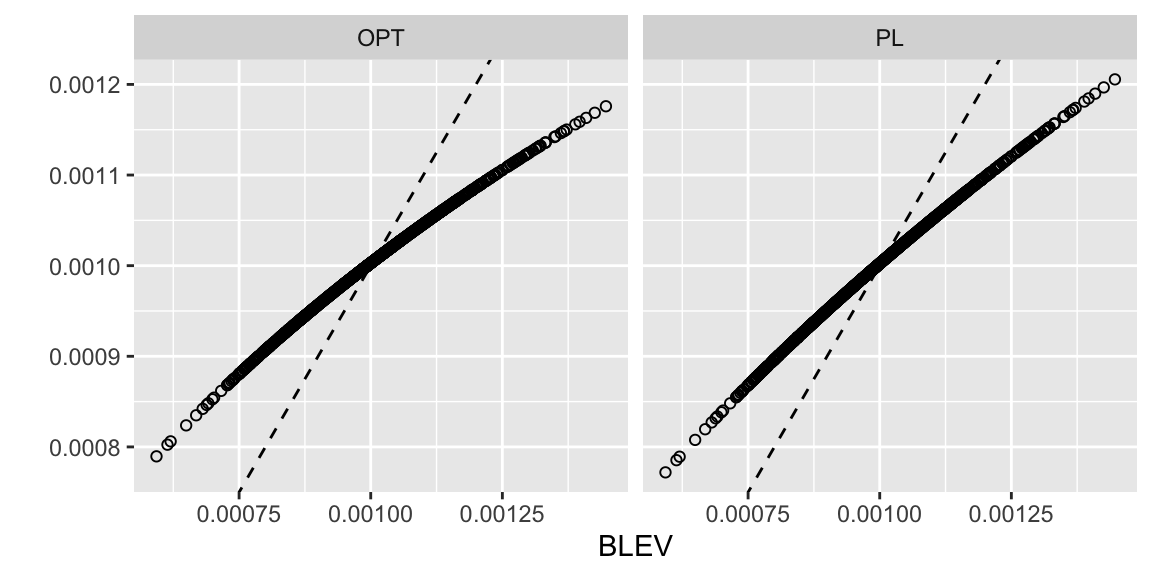
Figure 10.3: Comparison of subsampling probabilities.
10.3 Linear regression model
10.3.1 A review of Zhu et al. (2015)
To illustrate the improvements associated with the methods proposed in Zhu et al. (2015), we will briefly replicate their main empirical findings here. The evaluate the performance of the different methods we will proceed as follows:
Empirical exercise
- Generate synthetic data \(\mathbf{X}\) of dimension \((n \times m)\) with \(n>>m\).
- Set some true model parameter \(\beta=(\mathbf{1}^T_{\overline{m*0.6}},\mathbf{1}^T_{\underline{m*0.4}})^T\).
- Model the outcome variable as \(\mathbf{y}=\mathbf{X}\beta+\epsilon\) where \(\epsilon \sim \mathcal{N}(\mathbf{0},\sigma^2 \mathbf{I}_n)\) and \(\sigma=10\).
- Estimate the full-sample OLS estimator \(\hat\beta_n\) (a benchmark estimator of sorts in this setting).
- Use one of the subsampling methods to estimate iteratively \(\{\hat\beta^{(b)}_m\}^B_{b=1}\). Note that all subsampling methods are stochastic so \(\hat\beta_m\) varies across iterations.
- Evaluate average model performance of \(\hat\beta_m\) under the mean-squared error criterium: \(MSE= \frac{1}{B} \sum_{b=1}^{B} MSE^{(b)}\) where \(MSE^{(b)}\) corresponds to the in-sample estimator of the mean-squared error of the \(b\)-th iteration.
This exercise - and the once that follow - are computationally expensive. For them to be feasible we have to refrain from bias-correcting the in-sample estimator of the MSE (see appendix for session info). We will use a simple wrapper function to implement the empirical exercise in R.
As in Zhu et al. (2015) we will generate the design matrix \(\mathbf{X}\) from 5 different distributions: 1) Gaussian (GA) with \(\mathcal{N}(\mathbf{0},\Sigma)\); 2) Mixed-Gaussian (MG) with \(0.5\mathcal{N}(\mathbf{0},\Sigma)+0.5\mathcal{N}(\mathbf{0},25\Sigma)\); 3) Log-Gaussian (LN) with \(\log\mathcal{N}(\mathbf{0},\Sigma)\); 4) T-distribution with 1 degree of freedom (T1) and \(\Sigma\); 5) T-distribution as in 4) but truncated at \([-p,p]\). All parameters are chosen in the same way as in Zhu et al. (2015) with exception of \(n=1000\) and \(p=3\), which are significantly smaller choices in order to decrease the computational costs. The corresponding densities of the 5 data sets are shown in Figure 10.11 in the appendix.
We will run the empirical exercise for each data set and each subsampling method introduced above. Figure 10.4 shows logarithms of the sampling probabilities corresponding to the different subsampling methods (UNIF not shown for obvious reasons). The plots look very similar to the one in Zhu et al. (2015) and is shown here primarily to reassure ourselves that we have implemented their ideas correctly. One interesting observation is worth pointing out however: note how the distributions for OPT and PL have lower standard deviations compared to BLEV. This should not be altogether surprising since we already saw above that for orthogonal design matrices the former methods inflate small leverage scores while shrinking high scores. But it is interesting to see that the same appears to hold for design matrices that are explicitly not orthogonal given our choice of \(\Sigma\).
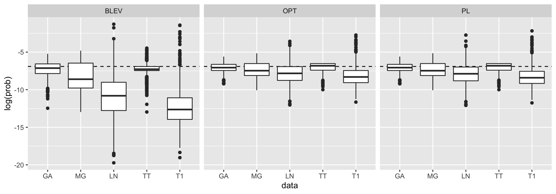
Figure 10.4: Sampling probabilities for different subsampling methods.
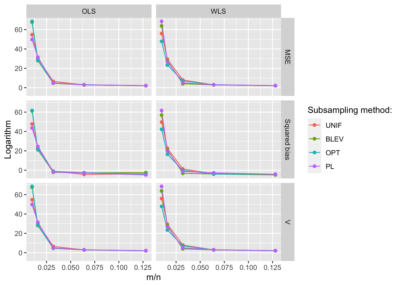
Figures 10.5 and 10.6 show the resulting MSE, squared bias and variance for the different subsampling methods and data sets using weighed least-squares and ordinary least-squares, respectively. The subsampling size increases along the horizontal axis. The figures are interactive to allow readers to zoom in etc.
For the data sets that are also shown in Zhu et al. (2015) we find the same overall pattern: PL and OPT outperform other methods when using weighted least-squares, while BLEV outperforms other methods when using unweighted/ordinary least-squares.
For Gaussian data (GA) the differences between the methods are minimal since data points are homogeneous. A similar picture emerges when running the method comparison for the sinusoidal data introduced above (see appendix). In fact, Zhu et al. (2015) recommend to just rely on uniform subsampling when data is Gaussian. Another interesting observation is that for t-distributed data (T1) the non-uniform subsampling methods significantly outperform uniform subsampling methods. This is despite the fact that in the case of T1 data the conditions used to establish asymptotic consistency of the non-uniform subsampling methods in Zhu et al. (2015) are not fulfilled: in particular the fourth moment is not finite (in fact it is not defined).
Figure 10.5: MSE, squared bias and variance for different subsampling methods and data sets. Subsampling with weighted least-squares.
Figure 10.6: MSE, squared bias and variance for different subsampling methods and data sets. Subsampling with ordinary least-squares.
10.3.2 Computational performance
We have already seen above that theoretically speaking both BLEV and OPT subsampling are computationally more expensive than PL subsampling (with UNIF subsampling the least expensive). It should be obvious that in light of their computational costs \(\mathcal{O}(np^2)\) the former two methods do not scale well in higher-dimensional problems (higher \(p\)). Zhu et al. (2015) demonstrate this through empirical exercises to an extent that is beyond the scope of this note. Instead we will just quickly benchmark the different functions for non-uniform subsampling introduced above: sub_BLEV, sub_OPT, sub_PL for \(n=200\), \(p=100\). We are only interested in how long it takes to compute subsampling probabilities, and since for sub_UNIF all subsampling probabilities are simply \(\pi_i=1/n\) we neglect this here. Figure 10.7 benchmarks the three non-uniform subsampling methods. Evidently PL subsampling is computationally much less costly.
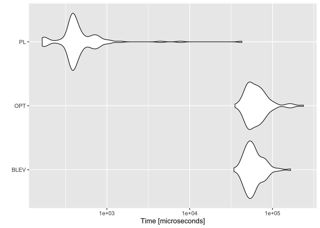
Figure 10.7: Benchmark of computational performance of different methods.
10.4 Classification problems
In binary classification problems we are often faced with the issue of imbalanced training data - one of the two classes is under-represented relative to the other. This generally makes classifiers less sensitive to the minority class which often is the class we want to predict (Branco, Torgo, and Ribeiro (2015)). Suppose for example we wanted to predict the probability of death for patients who suffer from COVID-19. The case-fatality rate for the virus is significantly lower than 10% so any data we could obtain on patients would inevitably be imbalanced: the domain is skewed towards the class we are not interested in predicting.
A common and straight-forward way to deal with this issue is to randomly over- or under-sample the training data. Let \(y_i\in{0,1}\) for all \(i=1,...,n\). We are interested in modelling \(p_i=P(y_i=1|x_i)\) but our data is imbalanced: \(n_{y=0}>>n_{y=1}\) where \(n=n_{y=0}+n_{y=1}\). Then random over- and under-sampling works as follows:
- Random oversampling: draw \(y_i\) from minority class \(\mathbf{y}_{n_{y=1}}\) with probability \(\{\pi_i\}^{n_{y=1}}_{i=1}=1/n_{y=1}\) and append \(\mathbf{y}_{n_{y=1}}\) by \(y_i\) so that \(n_{y=1} \leftarrow n_{y=1}+1\) until \(n_{y=0}=n_{y=1}\).
- Random undersampling: draw \(y_i\) from majority class \(\mathbf{y}_{n_{y=0}}\) with probability \(\{\pi_i\}^{n_{y=0}}_{i=0}=1/n_{y=0}\) and remove \(y_i\) from \(\mathbf{y}_{n_{y=0}}\) so that \(n_{y=0} \leftarrow n_{y=0}-1\) until \(n_{y=0}=n_{y=1}\).
In a way both these methods correspond to uniform subsampling (UNIF) discussed above. Random oversampling may lead to overfitting. Conversely, random undersampling may come at the cost of eliminating observations with valuable information. With respect to the latter, we have already shown that more systematic subsampling approaches generally outperform uniform subsampling in linear regression problems. It would be interesting to see if we can apply similar ideas to classification with imbalanced data. How exactly we can go about doing this should be straight-forward to see:
- Systematic undersampling: draw \(n_{y=1}\) times from from majority class \(\mathbf{y}_{n_{y=0}}\) with probability \(\{\pi_i\}^{n_{y=0}}_{i=0}\) defined by optimal subsampling methods and throw out the remainder.
To remain in the subsampling framework we will focus on undersampling here. It should be noted that many systematic approaches to undersampling already exist. In their extensive survey Branco, Torgo, and Ribeiro (2015) mention undersampling methods based on distance-criteria, condensed nearest neighbours as well as active learning methods. Optimal subsampling is not mentioned in the survey.
10.4.1 Optimal subsampling for classification problems
We cannot apply the methods used for subsampling with linear regression directly to classification problems, although we will see that certain ideas still apply. Wang, Zhu, and Ma (2018) explore optimal subsampling for large sample logistic regression - a paper that is very much related to Zhu et al. (2015). We will not cover the details here as much as we did for Zhu et al. (2015) and instead jump straight to one of the main results. Wang, Zhu, and Ma (2018) and propose a two-step algorithm that in the first step estimates logistic regression with uniform subsampling using \(m_0\) observations. In the second step the estimated coefficient \(\beta^{(UNIF)}_{m_0}\) from the first step is used to compute subsampling probabilities as follows:
\[ \begin{equation} \begin{aligned} && \pi_i&= \frac{|y_i-p_i(\beta^{(UNIF)}_{m_0})|||\mathbf{X}_i||}{\sum_{j=1}^n|y_i-p_i(\beta^{(UNIF)}_{m_0})|||\mathbf{X}_j||}\\ \end{aligned} (\#eq:subs_mVc) \end{equation} \]
The probabilities are then used to subsample \(m\) observations again. Finally, \(\hat\beta_{m_0+m}\) is estimated from the combdined subsamples with weighted logistic regression where weights once again correspond to inverse sampling probabilities. The authors refer to the method corresponding to @ref{eq:subs_mVc} as mVc since it corresponds to optimal subsampling with variance targeting. They also propose a method which targets the MSE directly, but this one is of higher computational costs \(\mathcal{O}(np^2)\) vs. \(\mathcal{O}(np)\) for mVc. The similarities to the case for linear regression should be obvious. We will only consider mVc here and see if it can be applied to undersampling. The code that implements this can be found here - it uses object-oriented program so could be interesting for some readers. Wang, Zhu, and Ma (2018) never run the model with ordinary as opposed to weighted logit, possibly because ordinary logit is not sensible in this context. But for the sake of completeness we’ll once again consider both cases here.
10.4.2 Synthetic data
In this section we will use the same synthetic data sets as above for our design matrix \(\mathbf{X}\). But while above we sampled \(y_i |x_i\sim \mathcal{N}(\beta^T x_i,\sigma)\), here we will simulate a single draw from \(\mathbf{y} |\mathbf{X} \sim \text{Bernoulli}(p)\), where in order to create imbalance we let \(p<0.5\) vary.
When thinking about repeating the empirical exercise from Section 10.3 above, we are faced with the question of how to compute the MSE and its bias-variance decomposition. One idea could be to compare the linear predictions in (7.3) in the same way as we did before, since after all these are fitted values from a linear model. The problem with that idea is that rebalancing the data through undersampling affects the intercept term \(\beta_0\) (potentially quite a bit if the data was originally very imbalanced). This is not surprising since \(\beta_0\) measures the log odds of \(y_i\) given all predictors \(\mathbf{X}_i=0\) are zero. Hence comparing linear predictors \(\mathbf{X}\beta_n\) and \(\mathbf{X}\beta_m\) is not a good idea in this setting (perhaps ever?). Fortunately though we can just work with the predicted probabilities in (7.2) directly and decompose the MSE in the same way as before (see Manning, Schütze, and Raghavan (2008), pp. 310):
\[ \begin{equation} \begin{aligned} && \mathbb{E} \left( (\hat{\mathbf{p}}-\mathbf{p})^2 \right) &= \text{var} (\hat{\mathbf{p}}) + \left( \mathbb{E} \left( \hat{\mathbf{p}} \right) - \mathbf{p} \right)^2 \\ \end{aligned} \tag{10.5} \end{equation} \]
Hence the empirical exercise in this section is very similar to the one above and can be summarized as follows:
Empirical exercise
- Generate synthetic data \(\mathbf{X}\) of dimension \((n \times m)\) with \(n>>m\).
- Randomly generate the binary outcome variable as \(\mathbf{y} | \mathbf{X} \sim \text{Bernoulli}(p=m/n)\).
- Estimate the full-sample logit estimator \(\hat\beta_n\).
- Use one of the undersampling methods to estimate recursively \(\{\hat\beta^{(b)}_m\}^B_{b=1}\).
- Evaluate average model performance of \(\hat\beta_m\) under the mean-squared error criterium: \(MSE= \frac{1}{B} \sum_{b=1}^{B} MSE^{(b)}\) where \(MSE^{(b)}\) corresponds to the in-sample estimator of the mean-squared error of the \(b\)-th iteration.
There is a decisive difference between this exercise and the one we ran for linear regression models above: here we are mechanically reducing the number of observations of the majority class and with non-uniform subsampling we are selective about what observations we keep. This is very different to simply subsampling without imposing a structure on the subsample. Intuitively it may well be that in this context non-uniform subsampling is prone to produce estimates of \(\hat\beta_m\) that are very different from \(\hat\beta_n\). This effect could be expected to appear in the squared bias term of the MSE.
The resulting mean-squared error decompositions are shown in Figures 10.8 and 10.9 for weighted and ordinary logit. A first interesting and reassuring observation is that both for weighted and ordinary logit the variance component is generally reduced more with mVc subsampling (certainly less true for weighted logit). A second observation is that the squared bias term can evidently not be controlled with mVc which leads to the overall mean-squared errors generally being higher than with random undersampling. This could be evidence that selective subsampling in fact introduces bias as speculated above, but this is not clear and would have to be explored more thoroughly.
It could also very well be that the algorithm in Wang, Zhu, and Ma (2018) was not implemented correctly here and the results are therefore incorrect. Unfortunately I have not had time to try and completely replicate that second paper also.
Figure 10.8: MSE, squared bias and variance for different subsampling methods and data sets. Subsampling with weighted logistic regression. MSE and its components correspond to linear predictions of logistic regression.
Figure 10.9: MSE, squared bias and variance for different subsampling methods and data sets. Subsampling with ordinary logistic regression. MSE and its components correspond to linear predictions of logistic regression.
10.4.3 Real data example
Until now we have merely looked at approximations of \(\hat\beta_n\) for logistic regression with imbalanced data. But ultimately the goal in classification problems is to accurately predict \(\mathbf{y}\) from test data. To investigate this point we will next turn to real data.
A number of interesting data sets related to COVID-19 have been made publicly available for research. An interesting data set for our purposes that contains information about individual patients is being maintained for the Open COVID-19 Data Working Group. The methodology for building the data set was originally developed by was developed by Xu et al. (2020). Information about how the data is being maintained and updated can be found in Group (2020). The complete data set is vast, but for our purposes we are only interested in the subset of data that contains information about the patient’s outcome state. The subset of the data we will use for our prediction exercise here is shown below. It contains the patient outcome variable \(y\in \{0=\text{survived}, 1=\text{deceased}\}\) which we are interested in predicting from a set of features: age, gender and geographical location. The model is kept intentionally simple, as our goal here continues to be the evaluation of subsampling methods, rather than building an accurate prediction.
The outcome variable is defined as \(y\in\{0=\text{survived},1=\text{deceased}\}\) and is highly imbalanced as expected: deaths make up about 4 percent of all outcomes. Note also that we are now looking at a significantly higher value for \(n\) than in the synthetic examples above. Computing leverage scores in this setting is extremely costly for reasons we have already elaborated on above and hence basic leveraging (BL) and optimal subsampling (OPT) are both omitted from the remainder of the analysis. To compare the two remaining approaches - uniform (UNIF) and prediction-length (PL) subsampling - we will proceed as follows:
To score our probabilistic predictions we will once again use the mean-squared error, although technically in this setting we would speak of the Brier score (see here):
\[ \begin{equation} \begin{aligned} && BS&= \frac{1}{n} \sum_{i=1}^{n} (p_i-\hat{p}_i)^2 \\ \end{aligned} \tag{10.6} \end{equation} \]
Of course other scoring functions are commonly considered for classification problems (for a discussion see for example here). But using the Brier score naturally continues the discussion above.
Empirical exercise
Cross-validate with \(k=5\) folds and for each fold repeat \(B=100\) times:
- Undersample the training data through one of the methods: \((\mathbf{X}_{\text{train}},\mathbf{y}_{\text{train}})\).
- Fit the model on the undersampled training data.
- Using the fitted model predict \(\hat{\mathbf{y}}_{\text{train}}\) using the test data \(\mathbf{X}_{\text{test}}\).
- Compute the Brier score for \(\mathbf{y}_{\text{test}}\) and \(\hat{\mathbf{y}}_{\text{train}}\).
Figure 10.10 shows the distribution of Brier scores resulting from our pseudo-out-of-sample predictions. Undersampling is performed both randomly and with mVc subsampling. The logit classifier is fitted separately with and without subsampling probabilities as weights. In the case of ordinary logit mVc seems to lead to slightly better predictions on average, but the improvement is not very significant. When the model is fitted with weights something interesting happens. The majority of the estimated Brier scores are lower than those obtained with random undersampling, but there is much higher variance and in some cases mVc performs very poorly. This could imply that using optimal subsampling for undersampling with weighted regression is risky: it performs well most of the time, but sometimes things go very wrong. Of course, this is a just a single example and the findings shown here are not sufficient to draw any conclusions.
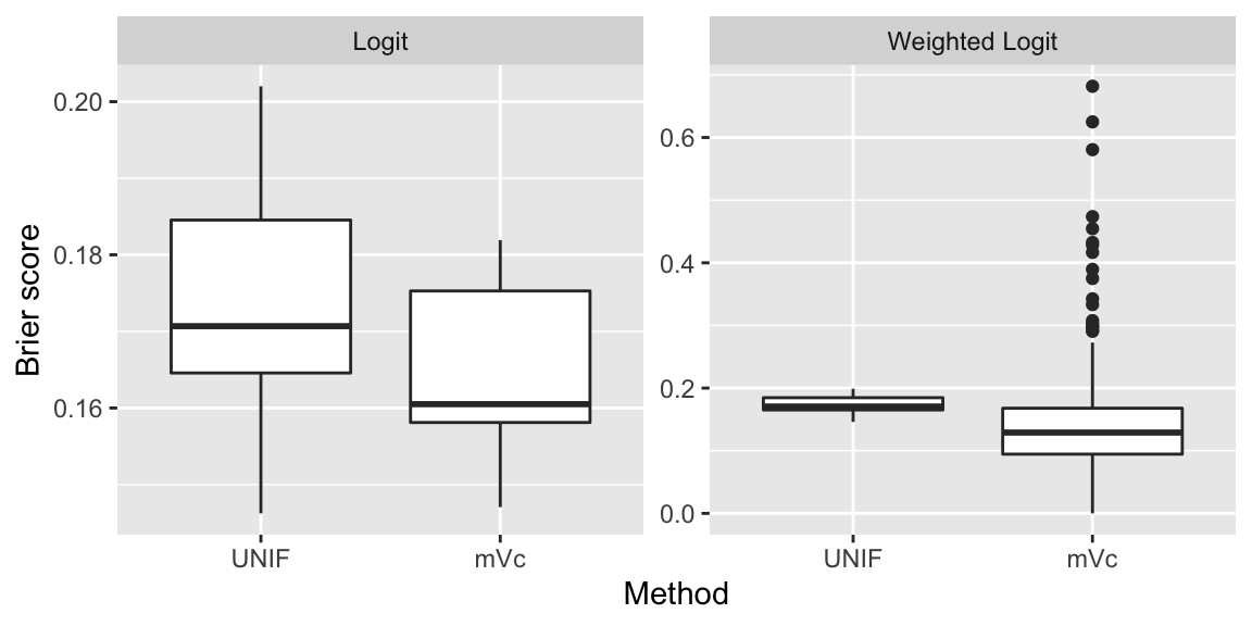
Figure 10.10: Distribution of Brier scores from pseudo-out-of-sample predictions for random and prediction-length undersampling.
10.5 Conclusion
In this short note we have looked at various systematic subsampling methods and how they can be applied to imbalanced learning. The fact that non-uniform subsampling can improve performance of linear regression models has been well established (Zhu et al. (2015)). We reviewed these findings here and then applied the developed idea to a binary classification problem with imbalanced data. The findings are mixed: it does appear that optimal subsampling methods can be successfully applied to undersampling in the sense that they can improve modely accuracy. While these findings are potentially interesting they are not conclusive. To establish general results theory would need to be developed. It is also far from clear whether the undersampling approaches presented here can compete with existing methodologies that involve distance-criteria, condensed nearest neighbours and active learning methods.
10.6 Appendix
10.6.1 From SVD to leverage scores
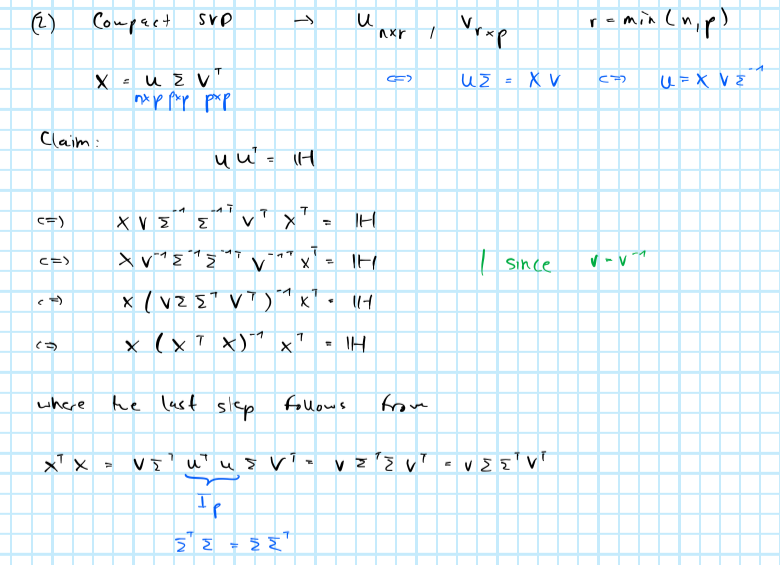
From SVD to leverage
10.6.2 From optimal to prediction-length subsampling
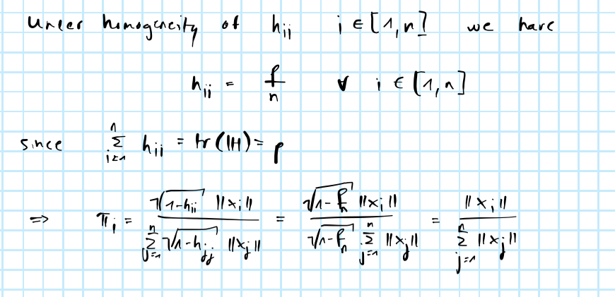
From OPT to PL
10.6.3 Synthetic data
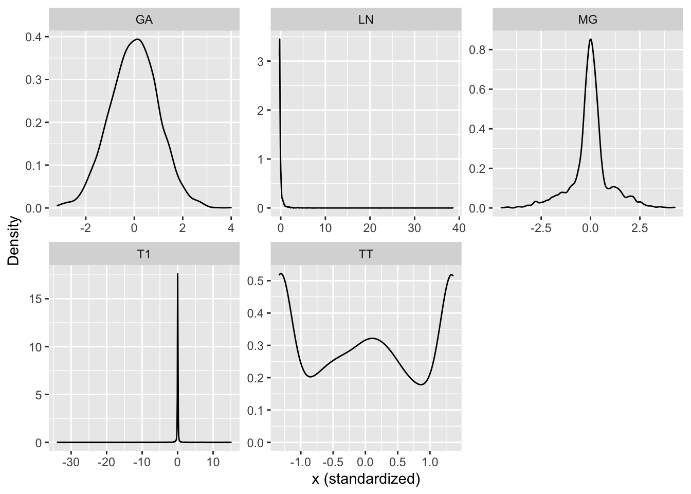
Figure 10.11: Densities of synthetic design matrices.
10.6.4 Subsampling applied to sinusoidal function