Chapter 2 Concentration inequalities
In order to measure the quality of an estimator we generally aim to minimize the expected value of a loss function \(\ell(x,y)\). Examples include:
- Mean squared error (MSE)
\[ \begin{equation} \begin{aligned} && \ell(x,y)=(x-y)^2 &\rightarrow \mathbb{E} \left[ \ell(x,y) \right] = \mathbb{E} (x-y)^2\\ \end{aligned} \tag{2.1} \end{equation} \]
- Mean absolute error (MAE)
\[ \begin{equation} \begin{aligned} && \ell(x,y)=|x-y| &\rightarrow \mathbb{E} \left[ \ell(x,y) \right] = \mathbb{E} |x-y|\\ \end{aligned} \tag{2.2} \end{equation} \]
More generally it is often useful to write:
\[ \begin{equation} \begin{aligned} && \ell(x,y)= \mathbb{1}_{|x-y|>\varepsilon} &\rightarrow \mathbb{E} \left[ \ell(x,y) \right] = P(|x-y|>\varepsilon)\\ \end{aligned} \tag{2.3} \end{equation} \]
2.1 Empirical mean
Let \(m\) denote the true value we want to estimate and \(m_n\) the corresponding estimator. An obvious choice for \(m_n\) is the empirical mean
\[ \begin{equation} \begin{aligned} && m_n&= \frac{1}{n} \sum_{i=1}^{n} x_i\\ \end{aligned} \tag{2.4} \end{equation} \]
for which we have
\[ \begin{equation} \begin{aligned} && \mathbb{E} \left[ m_n\right]&= \mathbb{E} \left[ \frac{1}{n} \sum_{i=1}^{n} x_i \right] = \frac{1}{n} \sum_{i=1}^{n} \mathbb{E} \left[x_i \right]=m\\ \end{aligned} \tag{2.5} \end{equation} \]
where the last equality follows from the law of large numbers. For the MSE of the empirical mean we have
\[ \begin{aligned} && \mathbb{E} \left[ m_n-m \right]^2 &= \mathbb{E} \left[ \frac{1}{n} \sum_{i=1}^{n} x_i-m \right]^2\\ && &= \mathbb{E} \left[ \frac{1}{n} \sum_{i=1}^{n} (x_i-m) \right]^2\\ && &= \frac{1}{n^2}\mathbb{E} \left[ \sum_{i=1}^{n} x_i-m \right]^2\\ && &= \frac{1}{n^2} n\text{var}(x_i)\\ \end{aligned} \]
and hence:
\[ \begin{equation} \begin{aligned} && \mathbb{E} \left[ m_n-m \right]^2&= \frac{\sigma^2}{n}\\ \end{aligned} \tag{2.6} \end{equation} \]
In other words, the size of the error is typically on the order of \(\frac{\sigma}{\sqrt{n}}\): the error decreases at a rate of \(\sqrt{n}\). Note that for the expected value of the mean absolute error we have \(\mathbb{E} |m_n-m| \le \sqrt{\mathbb{E} \left[ m_n-m \right]^2} =\frac{\sigma}{\sqrt{n}}\) by the Schwartz inequality.
What about \(P(|x-y|>\varepsilon)\), the third measure of expected loss we defined in (2.3)?
2.2 Simple non-asymptotic concentration inequalities
2.2.1 Markov’s inequality
2.2.2 Chebychev’s inequality
Applying Chebychev to the empirical mean we can show:
By ?? we have that with probability \(1-\delta\): \(|m_n-m|\le \frac{\sigma}{\sqrt{n\delta}}\). This can be shown as follows: if we want to guarantee that
\[ \begin{aligned} && P(|m_n-m|>\varepsilon)&\le \delta\\ \end{aligned} \]
then by ?? it suffices that:
\[ \begin{aligned} && \frac{\sigma^2}{n\varepsilon^2}&\le \delta \\ \end{aligned} \] This holds if:
\[ \begin{aligned} && \frac{\sigma}{\sqrt{n\delta}}&\le \varepsilon\\ \end{aligned} \]
2.3 Asympotic concentration inequalities
2.3.1 Central Limit Theorem
By the Central Limit Theorem we have that
\[ \begin{aligned} && P \left( \sqrt{n} \left( \frac{1}{n} \sum_{i=1}^{n} x_i-m\right) \ge t \right)& \rightarrow P(z \ge t) \le 2 \exp(- \frac{t^2}{2\sigma^2}) \\ \end{aligned} \]
where \(z \sim \mathcal{N}(0,\sigma^2)\). Letting \(\varepsilon = \frac{t}{\sqrt{n}}\) we have that asymptotically
\[ \begin{aligned} && P \left( \sqrt{n} \left( \frac{1}{n} \sum_{i=1}^{n} x_i-m\right) \ge \varepsilon \right)& \le 2 \exp(- \frac{\varepsilon^2n}{2\sigma^2}) \\ \end{aligned} \]
which is a much tigher bound than for example Chebychev.
2.4 Exponential non-asymptotic concentration inequalities
The motivation for deriving tight non-asymptotic concentration inequalities is that often we have \(d >> n\). In those case we want to control the worst error across all estimators (here the \(1,...,d\) empirical means). Hence our goal is to minimize
\[ \begin{aligned} && P( \max_j|m_{n,j}-m|\ge \varepsilon) \\ \end{aligned} \]
By the union bound we have
\[ \begin{aligned} && P( \max_j|m_{n,j}-m|\ge \varepsilon)&\le \sum_{j=1}^{d} P( |m_{n,j}-m|\ge \varepsilon)\\ \end{aligned} \]
and by Chebychev (??):
\[ \begin{aligned} && \sum_{j=1}^{d} P( |m_{n,j}-m|\ge \varepsilon)&\le d \frac{\sigma^2}{n\varepsilon^2}\\ \end{aligned} \]
Clearly, if \(d>>n\) we are in trouble. Enter: Chernoff bounds.
2.4.1 Chernoff bounds
2.4.2 Hoeffding’s Inequality
Using Hoeffding’s Lemma (??) and Chernoff’s bounds (??) we get Hoeffding’s inequality:
2.4.3 Bernstein’s inequality
2.5 Examples
Finally, let us at a few examples. Firstly, let us look at what bounds we get for the different concentration inequalities when applied to the binomial distribution:
Another illustrative application of Chernoff’s bounds emerges in the context of high-dimensional spaces. Consider the question of how many points we can choose on the \(d\)-dimensional unit ball, such that their pair-wise angles are (almost) orthogonal.
Hence, if \(d \ge \frac{5.5451774}{\varepsilon^2}\) we can choose \(n= e^{ \frac{d \varepsilon^2}{8}}\) points such that their pair-wise almost orthogonal.
2.6 Appendix
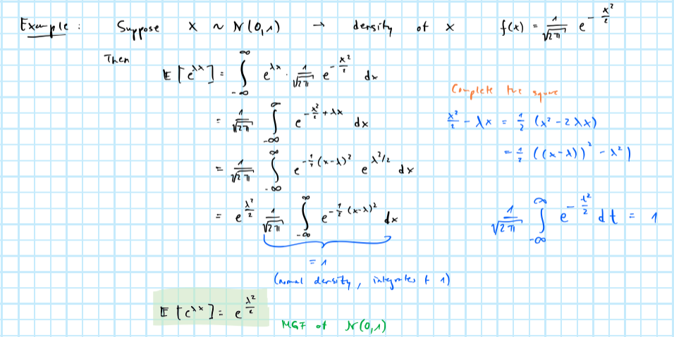
2.6.1 Example of a moment generating function