Chapter 7 Regression
7.1 Ordinary least-squares
Both OLS and WLS are implemented here using QR decomposition. As for OLS this is very easily done in R. Given some feature matrix X and a corresponding outcome variable y we can use qr.solve(X, y) to compute \(\hat\beta\).
7.2 Weighted least-squares
For the weighted least-squares estimator we have: (see appendix for derivation)
\[ \begin{equation} \begin{aligned} && \hat\beta_m^{WLS}&= \left( \mathbf{X}^T \Phi^{-1} \mathbf{X} \right)^{-1} \mathbf{X}^T\Phi^{-1}\mathbf{y}\\ \end{aligned} \tag{7.1} \end{equation} \]
In R weighted this can be implemented as follows:
function (X, y, weights = NULL)
{
    if (!is.null(weights)) {
        Phi <- diag(weights)
        beta <- qr.solve(t(X) %*% Phi %*% X, t(X) %*% Phi %*% y)
    }
    else {
        beta <- qr.solve(X, y)
    }
    return(beta)
}
7.3 Logisitic regression
To model the probability of \(y=1\) we will use logistic regression:
\[ \begin{equation} \begin{aligned} && \mathbf{p}&= \frac{ \exp( \mathbf{X} \beta )}{1 + \exp(\mathbf{X} \beta)} \end{aligned} \tag{7.2} \end{equation} \]
Equation (7.2) is not estimated directly but rather derived from linear predictions
\[ \begin{equation} \begin{aligned} \log \left( \frac{\mathbf{p}}{1-\mathbf{p}} \right)&= \mathbf{X} \beta \\ \end{aligned} \tag{7.3} \end{equation} \]
where \(\beta\) can be estimated through iterative re-weighted least-squares (IRLS) which is a simple implementation of Newton’s method (see for example Wasserman (2013); a complete derivation can also be found in the appendix):
\[ \begin{equation} \begin{aligned} && \beta_{s+1}&= \left( \mathbf{X}^T \mathbf{W} \mathbf{X} \right) \mathbf{X}^T \mathbf{W}z\\ \text{where}&& z&= \mathbf{X}\beta_{s} + \mathbf{W}^{-1} (\mathbf{y}-\mathbf{p}) \\ && \mathbf{W}&= \text{diag}\{p_i(\beta_{s})(1-p_i(\beta_{s}))\}_{i=1}^n \\ \end{aligned} \tag{7.4} \end{equation} \]
In R this can be implemented from scratch as below. For the empirical exercises we will rely on glm([formula], family="binomial") which scales much better to higher dimensional problems than my custom function and also implements weighted logit.
function (X, y, beta_0 = NULL, tau = 1e-09, max_iter = 10000)
{
    if (!all(X[, 1] == 1)) {
        X <- cbind(1, X)
    }
    p <- ncol(X)
    n <- nrow(X)
    if (is.null(beta_0)) {
        beta_latest <- matrix(rep(0, p))
    }
    W <- diag(n)
    can_still_improve <- T
    iter <- 1
    while (can_still_improve & iter < max_iter) {
        y_hat <- X %*% beta_latest
        p_y <- exp(y_hat)/(1 + exp(y_hat))
        df_latest <- crossprod(X, y - p_y)
        diag(W) <- p_y * (1 - p_y)
        Z <- X %*% beta_latest + qr.solve(W) %*% (y - p_y)
        beta_latest <- qr.solve(crossprod(X, W %*% X), crossprod(X, W %*% Z))
        can_still_improve <- mean(abs(df_latest)) > tau
        iter <- iter + 1
    }
    return(list(fitted = p_y, coeff = beta_latest))
}
7.4 Appendix
7.4.1 Weighted least-squares
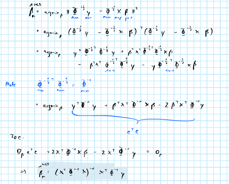
Weighted least-squares
7.4.2 Iterative reweighted least-squares
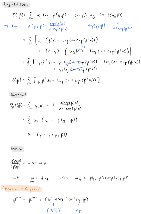
Iterative reweighted least-squares